EARTHQUAKE HAZARD
AND SEISMIC RISK (EGU-GIFT 2013-2017-2022)
|
|
XII) MOVEMENTS of the 2 sides of a fault studied
with AZIMUT and SISMO BOX |
|
|
VIII) LOCATION determination of an eathquake
and wave speed in the crust |
|
|
|
I) OVERVIEW VIDEOS
![]() LINK TO ALL
FILMS YOUTUBE INTEGRATED
LINK TO ALL
FILMS YOUTUBE INTEGRATED
|
|
|
|
|
|
|
|
|
|
Sismo
box |
Seismometer |
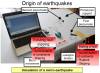
Earthquake’s
origin |
Eathquake
prediction |
Resonance |
Resonance
at 3l/4 |
Ground
liquefaction |
Site
effect excentric |
|
|
|
|
|
|
|
|
|
|
Site
effect Grenoble |
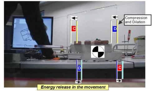
Energy
accumulation |
Energy
accumulation |
Bearing
wall |
Roof
amortissement |
Shake
table |
Switch
el. Screw-driver |
Using
excentric |
|
|
|
|
|
|
|
|
|
|
Electronic
shake table |
Azimut
software |
|
|
|
|
|
|


II) RISK
EQUATION and shown elements with SISMO BOX 
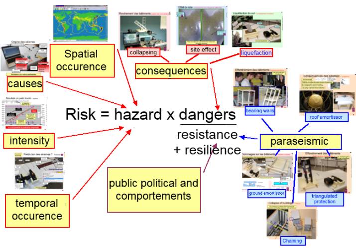 Source: UVED modified
Seismic
hazard is defined by earthquakes causes (global geology), spatial and
temporal occurrence, intensity. With the sismo box, man can show that it is
possible to predict the location of an eathquake, but neither it’s intensity,
nor it’s occurrence.
The risk
depends of the hasard, and of the consequences on human lifes and activities.
It is decreases by the resistance with paraseismic systems, and the
resilience wich measure the capacity to limit it’s consequences.
It
depends of the human comportments and public politicals.
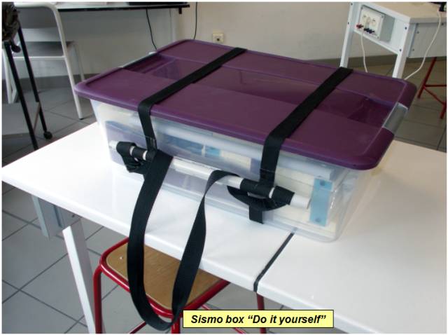
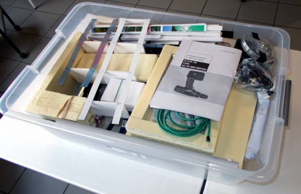
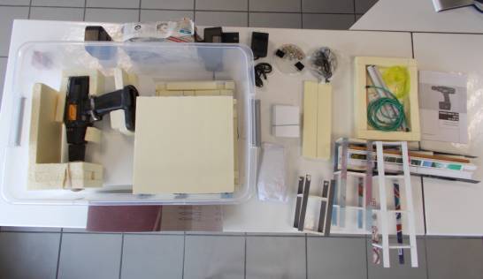
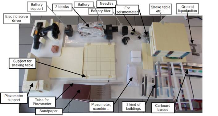
III) THE SISMO BOX “DO IT
YOURSELF” ![]()
|
|
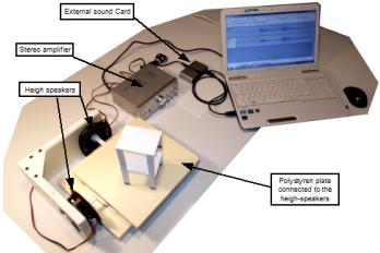
IV) ADDITIONAL EQUIPMENT TO MAKE
A 1D-2D ELECTRONIC TABLE
![]()
|
|

|
|
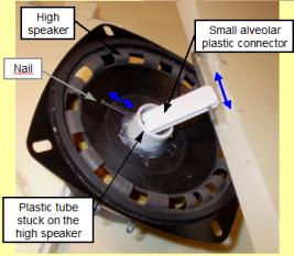
Necessary equipment to make this experiment:
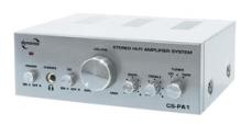
(Conrad) Dynavox mini-ampli Hi-Fi CSPA1 silver ref :76001
1 F7 39,90 € 2*High
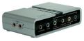
speakers SPEAKA HP 75-9 ref: 300237 1 F7 2*12,95 € USB
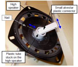
external sound card 7.1 USB2.0 ref: 87176 1 F7 39,95 € The high speaker can be perforated to
increase the movement amplitude, but the external sound-card is very
efficient, particulary with laptop computers. The main interest using a
electronic shaking table, is to send to the table a real earthquake trace,
and to approach the reality. In a real trace, all frequencies as present
and the building resonance shows that phenomenon. |
V) HOW AND WHY RECORDING
EARTHQUAKES
![]()
|
|
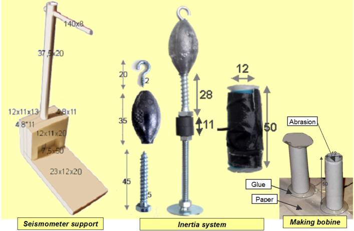
How
to build a sismometer:
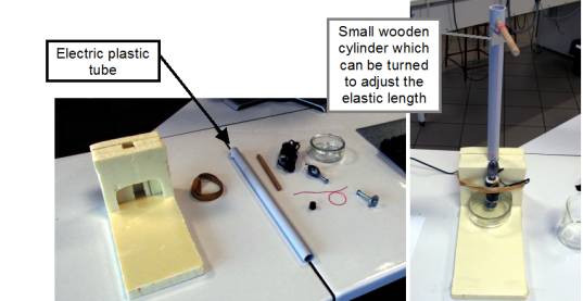
Principle: record the relative movement of
the earth compare with something immovable.
Ground
vibrations are recorded by the relative movement of a magnet in a bobine
(Induction)
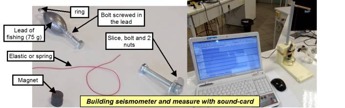
The mass
is considered as inmovable (inertia) and is hang with an elastic.
The
movement of the mass after the earth vibration must be weakened by the slice
wich is in the water.
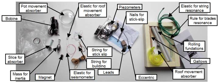
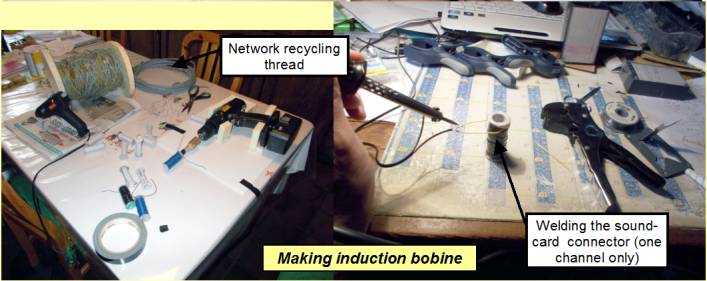
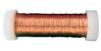
Material: Tube, polystyren support,
elastic, masse, magnet, pot with water, slices, bobine connected to Audacity,
with external entry, and one channel.
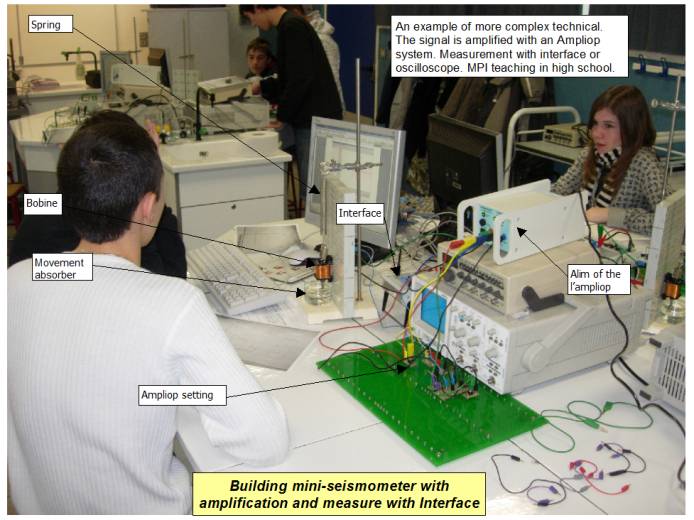
Experiment: The polystyren must be stick on
the earth support (table). Try the efficacity of the amortissement by lifting
the mass then by dropping it.
Students
can draw the system with 2 colors; one for what is moving in case of
earthquake, and an other to draw what don’t move in case of earthquake.
Important
remarks: In all
cases, you have to get maximum amplify. (on certain computers, amplification
of sound-card is to low to see convincing things)
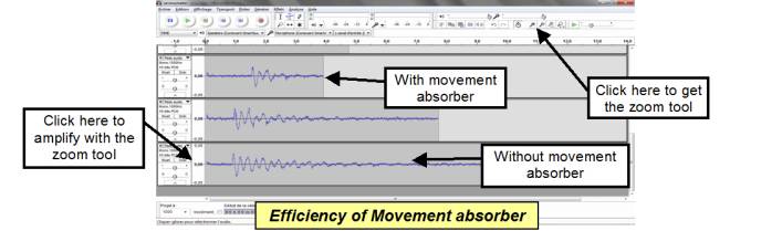
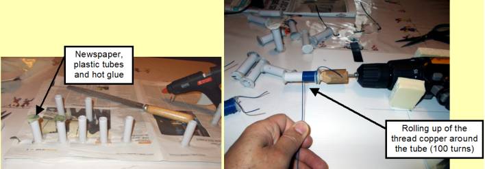
The
bobine has approximately 100 tours, so the induction current is not so
important. If you chock the table you can register something, but you have to
amplify at maximum.
How to build yourself?
Polystyren can be cut with jig-saw or cutter
and glue with a heater glue gun. Network thread recycling.
|
|
The
inertia principle of Isaac Newton is used to undertand how a mass hung on a
spring remains ephemerally immovable when the ground moves during an
earthquake, and allows its recording.
|
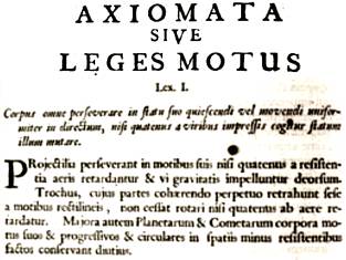
Philosophiae Naturalis Principia Mathematica, 1686. Isaac
Newton (1642-1727) AXIOMATA SIVE LEGES MOTUS Lex I: Corpus
omne perseverare in statu suo quiescendi vel movendi uniformiter in
directum, nisi quatenus a viribus impressis cogitur statum illum mutare. Projectilia
perseverant in motibus suis nisi quatenus a resistentia aeris retardantur
& vi gravitatis impelluntur deorsum. Trochus, cujus partes cohaerendo
perpetuo retrahunt sese a motibus rectilineis, non cessat rotari nisi
quatenus ab aere retardatur. Majora autem Planetarum & Cometarum
corpora motus suos & progressivos & circulars in spatiis minus
resistentibus factos conservant diutius.
Latina text of Newton 1st
movement law |
|
Law I.
Every
body perseveres in its state of rest, or of uniform motion in a right line,
unless it is compelled to change that state by forces impressed thereon.
Projectiles
continue in their motions, so far as they are not retarded by the resistance
of the air, or impelled downwards by the force of gravity. A top, whose parts
by their cohesion are continually drawn aside from rectilinear motions, does
not cease its rotations, otherwise than it is retarded by the air. The
greater bodies of the planets and comets, meeting with less resistance in
freer spaces, persevere in their motions both progressive and circular for a
much longer time. http://physics.info/newton-second/
|
|
|
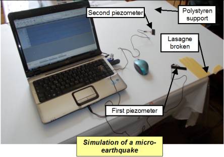
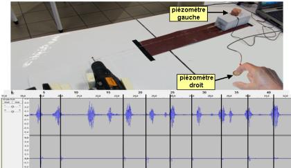
Principle: set an accumulation of energy
with a lasagne until it breaks. A wave goes away from the rupture location
and is recorded by the piezometer connect to Audacity. Material: lasagnes, one or 2 channels on
Audacity, one or two piezometers. Experiment: Run audacity and break the
lasagne: The disturbance goes around and stimulates the piezometer which
records it. The earthquake appears around the fault: propagation: (risk
exists even far from the earthquake). There is an amortissement with the
distance. |
|
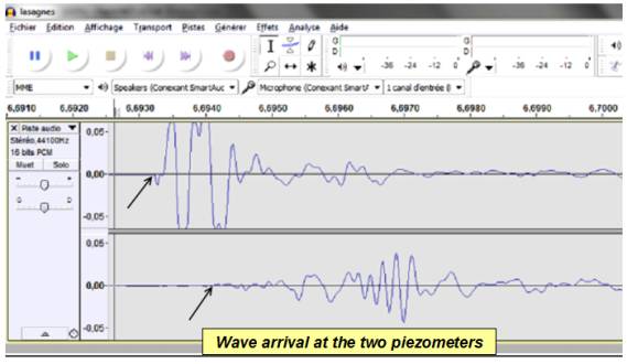
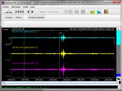
We can see the amortissement with the distance, also that the signal is complex.
Delta t is 0.7 ms for the wave to go from one piezometer to the other. (0.8 m): 1.1/1.2 km/s in the polystyren.
Important
remark:
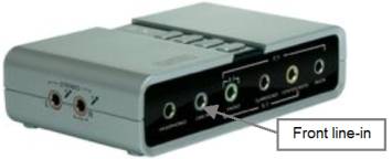
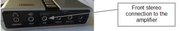
With
certain laptop computers, the card sound does not allow the stereo
acquisition. You have to get an external sound card ( Sweex: see below)
Connect
the stereo piezometer to the front line in, and select in Audacity “Line enter USB multi-channel” to active
the USB external sound card.
|
|
parameters
in audacity software |
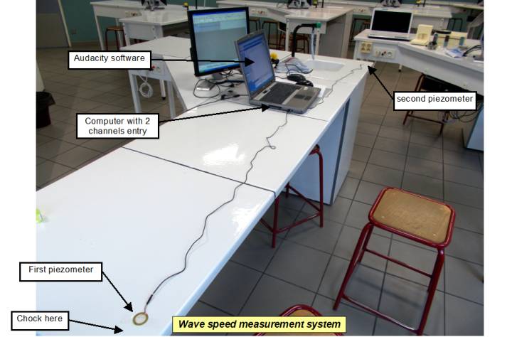
VII) MEASUREMENT OF THE SPEED OF THE
EARTHQUAKE’ S WAVES: ![]()
Principle: measurement of the earthquake
speed propagation in different materials.
Material: 2 channels on Audacity, two
piezometers, table in wood or concrete or polystyren piece.
The
experiment is
done with 2 pizometers and a chock with a hard piece of metal, or with a
pencil (on the polystyren)
Measurement
of different arrival times and distance between the 2 piezometers. (speed in concrete is ≈3.2 km/s)
in polystyren (≈1.2 km/s)
Wave
speed on the ground can be evaluate with Educarte software or Sismolog (see
below).
VIII) DETERMINATION OF THE
EARTHQAKE’S LOCATION AND WAVE SPEED: ![]()
2 methods
to locate near eathquakes: half plane (which can be
experimental too in the classroom) et S-P circle, when we know speed,
software Sismolog or Educarte.
Using
Sismolog (Chrysis)
author Julien FRECHET, François THOUVENOT (LGIT CNRS Grenoble) and the
SISMALP seismic network: problem is we don’t know where was the earthquake,
when took place the earthquake, et the speed of the wave. Once known the
earthquake’s position by the half – plans method, we know all the rest.
|
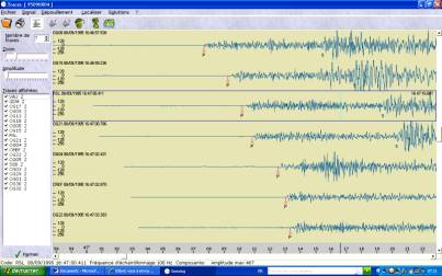
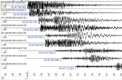
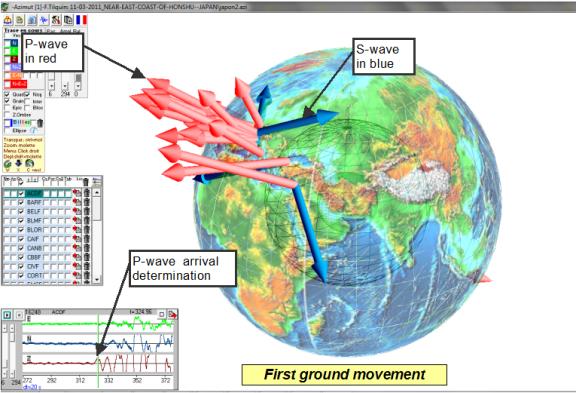
Arrival time of P-wave |
The
first work is to determine the arrival time of the P-waves and S-waves. |
||
|
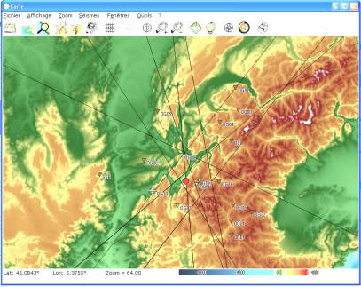
Half plane earthquake
location method |
The
method of the half-plans: we draw the mediator between 2 stations then we
consider that the earthquake is in the half-plan of the station having
received the wave P first. By taking stations 2 by 2 we determine a
polygon in which is the earthquake. The
software draws a shadow in the half-plane which do not contains earthquake
(not too visible here) Once
the position of the earthquake is known, we can calculate the wave speed
and t0. This
method can be used in clasroom (see below) |
||
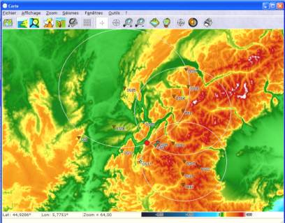
|
Circle S-P earthquake
location method |
The
method of circles is possible when the speed of the P-wave and S-wave is
known . We have
also to consider the depth of earthquake. It
seams the circles do not determine a precise point but a polygon when the
earthquake is not superficial, but deep: There is a difference in the
distance between the real route and the visible route of the waves. |
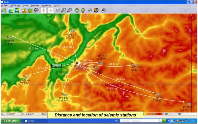
P-Wave
speed measurement on the ground with near earthquakes:
In this
example, the earthquake depth is 6.51 Km. Each station has an altitude, a
p-wave arrival time, a distance from epicenter which is calculate with GPS
coordinates.
|
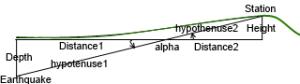
To know the distance traveled by the wave,
it is necessary to know the sum of 2 hypotenuses. Sin α=depth/hyp1=height/hyp2 and Cos
α=D1/hyp1=D2/hyp2 D1+D2=cos α(hyp1+hyp2) and
Depth+height= Sin α(hyp1+hyp2) Square and sum gives: (D1+D2 )2+(depth+height)2=cos2
α(hp1+hyp2)2+sin2 α(hp1+hyp2)2 ans the wave travel is: hyp1+hyp2=sqrt( (D1+D2 )2+(depth+height)2) The array below shows that the error is not
so big if we consider that the earthquake and station are at the zero
level. |
Seismogram and p-wave arrival time Earthquake depth is 6,51 km
S |

|
Station |
Height (km) |
Distance D1+D2 (km) |
Distance wave Hyp1+hyp2 |
Arrival time (h:min:sec) |
Delta d (km) |
Delta t (s) |
p-wave speed (km/s) |
|
OG08 |
0,550 |
59,92 |
60,33 |
16:47:07.658 |
|
|
|
|
OG09 (-OG08) |
0,630 |
34,86 |
35,58 |
16:47:03.345 |
24,75 |
4,313 |
5,73 |
|
OG13 (-OG08) |
0,560 |
42,39 |
42,97 |
16:47:04.702 |
17,36 |
2,956 |
5,87 |
|
OG18 |
1,455 |
40,89 |
41,65 |
16:47:04.912 |
|
|
|
|
GDM (-OG18) |
1,574 |
16,3 |
18,19 |
16:47:00.561 |
23,46 |
4,351 |
5,39 |
|
OG15 |
1,985 |
66,6 |
67 |
16:47:09.246 |
|
|
|
|
(OG15-) VAU |
1,455 |
15,89 |
17,77 |
17:47:00.062 |
49,23 |
9,184 |
5,36 |
|
OG22 (-VAU) |
1,810 |
91,85 |
92,23 |
16:47:13.303 |
74,92 |
13,241 |
5,65 |
![]()
We can
observe some variations of the P-Wave and it is not really possible, at this
level, to find a law.
Earthquake
location in classroom, using microphones: a chock will be set: man do not know
neither the location of the earthquake, nor the speed of the wave.
Material
5-10 double piezometers with long connectors (3-5 meters for a classroom,
authorize the measurement of 6-10 meters)
One
piezometer is very near of the chock (zero time) and the others are anywhere
in the classroom.
The
difference between the 2 arrivals is collected in an array.
The
students have the map of the classroom and the differents piezometers are
ploted on it.
Audacity
must be with the maximum of point per second (96000 Hz) Edition, Preferences,
Qualité.
Each
group write on the blackboard the arrival time (difference beetween first
spike and second spike)
On the
individual map, students join station and draw mediator, then eliminate the
half plane which does not contain the earthquake.
They can
determine so, step by step, a polygon which contains the earthquake.
(précision 30 cm in the classroom)
When
earthquake location is determinate, it is also posible to have the wave
speed.
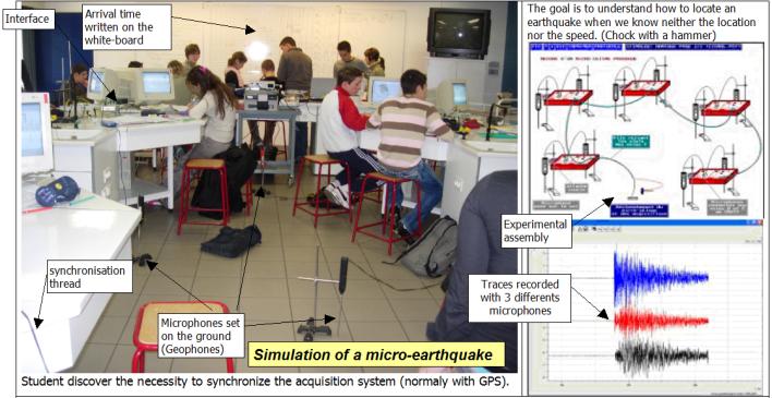
Aclassroom map is written
on the white board and arrival times to each station are red by the students
and writtent on the white-board. The half-plane method allows the location of
the eathquake with about 30 cm precision. The acquisition is made with a
frequency of 100000 Hz. (The speed wave in concrete is about 3.2 Km/s)
How to build yourself?
You can command the 2 elements on the website
http://www.conrad.fr
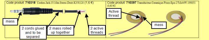
You have to separe the 2 mass connectors which are rolled up together, and separe
the 2 cords glued together. Weld the 2 mass of the connector to the mass of
the 2 piezometers and make and weld the 2 active threads to the 2 active
threads of the piezometer. Roll up the connection to strengthen.
Earthquake
location in classroom using piezometers: without synchronisation.
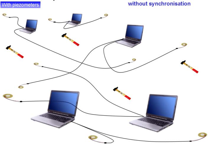
No
synchronisation
between computers: we have only 5 mediators for 5 computers. Low precision in
drawing the polygon wich contains earthquake.
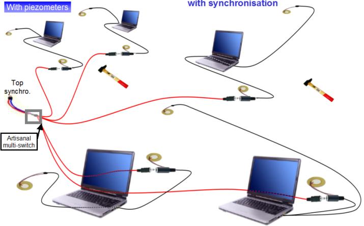
With
the top-synchro:
50 mediators with 5 computers. Signal synchro can be a small electric
tension, with an artisanal multi-switch wich disconnect each computer after
the top synchonisation.
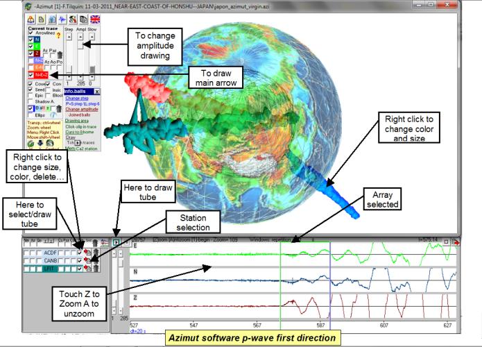
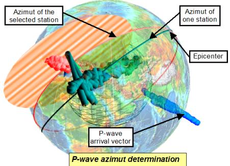
Location far earthquakes: azimutal
method Japan earthquake. Software AZIMUT©FT Free
|
|
After
running choose language, then right click, read selected position, directory
japan, japan_azimut_virgin, place cursor near P-wave arrival, and Z to zoom,
select the array of p-wave during about 20 seconds (click and slip), change
eventually the amplitude of the signal in clicking in the selected array and
look red arrow (in this example, amplitude 285 is good) , then put the reading cursor at the
beginning of the array selected (button home), click on the check
corresponding to “tub” on the windows left of the station name, and run the
trace: tube appears , drawing extremity of the main arrow.
Do this
for the other stations ( red arrow in the station window to select the new
station)
|
After
drawing tubes, you have to place the azimut: in the gray windows left top,
click on check Az and Paz: an orange circle appears on the select station:
3 proximal keys M, %, µ use with the mouse wheel to change Azimut, change
size, change transparency. The
orange plane must split points in 2 equal parts. Normaly
the 3 azimut stations show the epicenter. |
|
World
location of earth quakes: Educarte (freeware) or Sismolog
Earthquake
hazard, and if when populations leave near, we can speak about earthquake
risk.
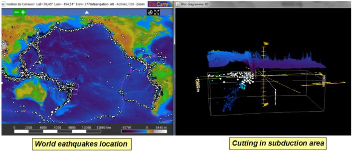
Educarte
software (J.L. Berenguer, A.Lomax) World sismicity and cut defined to show
Benioff plan.
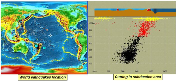
Sismolog
software (J.Frechet, F.Thouvenot LGIT Grenoble)
With
Sismolog, we can change the width of the cut: earthquake are thrown on the
middle line. The cut must be very perpandiculary to the Benioff plan, and it
is then possible to measure the width of the lithospheric plate.
IX) EARTHQUAKES PREDICTION ?
WHERE, WHEN, HOW ? ![]()
|
|
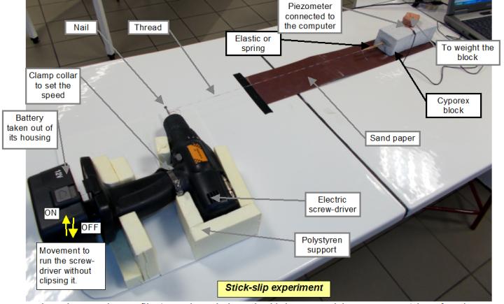
Stick
slip experiment with sismo-box “do it yourself” (sand paper, electric screewdriver
with slow speed, elastic, rock block).
|
|
Stick
slip experiment with step to step engine, sand paper, elastic, rock block).
|
|
Very
simple device for the stick slip experiment.
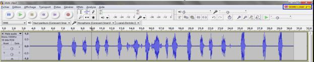
Software ![]() sets the good parameters of
audacity. If it does not run set the parameters of audacity to 1
channel, 1000 hz, 16 bits. Experiment
time: 30 second max. (because of the Excel number of point limits.
sets the good parameters of
audacity. If it does not run set the parameters of audacity to 1
channel, 1000 hz, 16 bits. Experiment
time: 30 second max. (because of the Excel number of point limits.
At
the end, export the wav file, (normaly Audacity make this in personnal
documents etc…) just after, sismo-logic read this new file automatically and
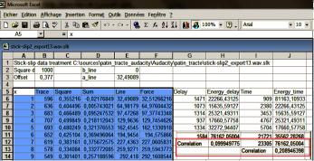
convert it in excel file, with formula, and run Excel.
|
Select the data from x until « Force » with shift and right-arrows and with «Ctrl» + «shift» + «down-arrow». Then go to the top with the lift and draw with “points cloud”
|
|
Change the slope and the shift of the blue line with a_droite
and b_droite parameters to put it in the right position. Then it is possible
to understand the difference between the theoretical and effective movement.
(Possibility of using 2 channel to try to
ask an user to hit on the second piezometer just before the slipping)
Possibility
to draw with a pencil the positions, and to put it in excel.
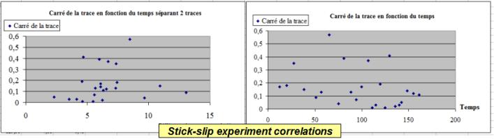
Measurement
the time between 2 slippings:
Try to
correlate with the energy of the most recent slipping (energy is
proportionnal to the square of the slipping trace= a sort of kinetic energy ½
m*v2).
How
to treat data to plot relation between slipping interval and energy.
By leaving of the intuitive hypothesis that more it
has been a long time since an earthquake took place, more the released energy
is strong, we are going to concern a graph the time separating two movements
and the energy of the earthquake. If there is a correlation, we should see
points getting organized according to a right.
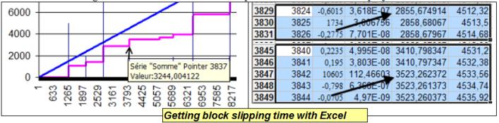
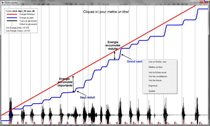
The principle is to study the picture of the curve in
staircase and to locate the moment when begins the step and the height of
this one.
By placing the mouse without clicking the curve in
staircase at the time of projections, appears the information allowing to
find the values of time in the
picture and the value of the projection.
|
|
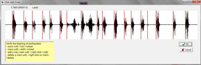
After sctick-slip wave file exportation, the software Sismo-lgic,
ask to the user to verify the beginning of each earthquake (red line) and
creates 2 new array: delay/ energy and time/energy. Correlation coefficient
are calculated. |
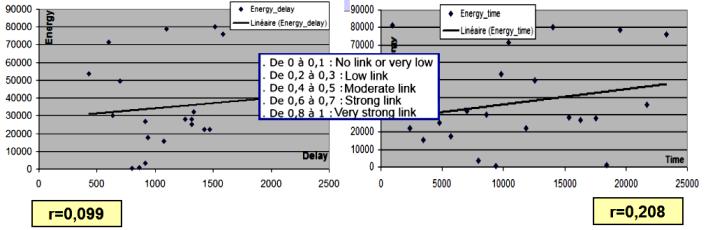
Results of the treatment energy-time separating two movements.
There is nothing really visible, although it seems to
take shape a kind of cloud of points.
It seems to have a small correlation (0,208) between the time and the energy,
because of the experimental protocole: the sand paper is more slippy at the
beginning because we made a lot of small experiment for the development.
(hypothesis)
With Sismo-logic :
At the end of experiment, in
Audacitymake File; Export or Export the selection.
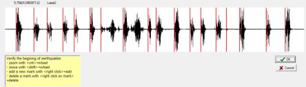
After
exportation, the sofware Sismo-Logic detects the presence of a new file .wav
in tge directory fic_sismo_logic\ Audacity\ patin_tracte and print the traces
with a red line before each beginning of sliping
|
|
|
It is necessary to verify that the software correctly
worked, and you can move the red lines according to the menu above. Once
after checking, click on OK to continue. |
Datas ar automaticaly treated :
A curve
appears, containing the tracks of the sliding, the energy actually restored
by the skate (curve in staircase), and the theoretical energy (just right
above).
Interpretations of the curves of waste of the
energy. (sismo-logic, Stick-slip
results)
L’énergie libérée par le patin est représenté par la
courbe en escalier (« Somme » des carrés de la trace).
The line
represents the theoretical energy (trend curve of the curve in staircase,
moved upward)
- We can characterize the time which separates two movements.
- The relations between the energy actually dissipated by the skate and the theoretical energy. Notion of delay in the balance.
- The relation between the magnitude and the delay in the
balance.
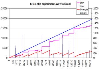
Traitement of the datas with Excel : The
access to the file is by the right click, then Seen the Excel file: it is
necessary to make then only draw the curve by Excel.
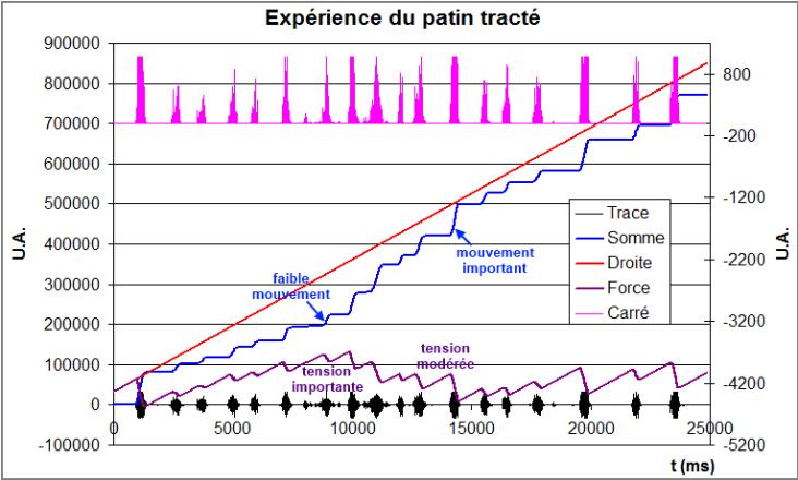
The purple peaks (at the top) represent the
"Square" of the track. The curve of the "Strength" is
obtained by subtracting the energy dissipated in the average right. We so
obtain the accumulation of energy and its liberation according to time. We
also notice that the sliding is not proportional in the present strength
before.
Treatement of data energy-delay between two
slippings.
The right click in
the previous curve allows to reach the correlations:
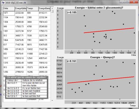
- We can, by using the box, characterize the correlation between the delay separating two earthquakes and the intensity of the second:
The Sismo-logic software
calculated the coefficient of correlation
" loose Energy ", " delay between 2 earthquakes ". In this example the coefficient
of correlation is 0 .016.
- We can finally
discuss the intuitive hypothesis that: " more it has been a long delay
between two earthquakes more the energy of the second is strong?
- The geologists speak about period of return to indicate the recurrence of certain earthquakes. We can calculate Under Excel, average of the time of occurrence of the sliding of the skate.
- We can also calculate the standard deviation which measures the dispersal and which can express itself in % :
the formula is =ecartypep (first line ; last line). The add p in the formula means that it is a small number of values.
NB : The field of lines is seized in the mouse by one to click to slide after the seizure of the opening parenthesis.
- By redoing the experience(experiment) several times and the calculations, we can discuss the notion of fluctuation in the sampling. see the file
- Try of seismic prediction.
|
- 2 piézometer are
necessary: the left one is going to record the sliping of the skate and the
right one the moment when you estimate to be just before this sliping, by
typing briefly above. - In sismo-logic, chose Audacity for stick slip prediction (Line in USB
multichannel, 2 channels, 22050 Hz). -
Make the experiment Proceed to the experience opposite; the experimentatorr
presses on his piezometer as soon as he believes that the skate is going to
move.See |
|
- The mode of mathematical treatment of these data is not immediate, because if the experimentator always types as the earthquake took place, we shall have a strong correlation.
Conclusions:
We can also make vary the roughness, the mass, the
steepness of the spring and show so that the more the friction is important,
the more the accumulated energy is important, and that more the ground is
elastic more the delay in the balance is important.
In every case, we can show that no sliding is predictable, good that we can
determine an average frequency.
We could think that numerous small earthquakes allow the
catching up, but curves show us that it is not really the case.
We do not see either forerunners of big earthquakes.
http://www.ac-grenoble.fr/webcurie/sismo/web_patin
X) CONSEQUENCES OF EARTHQUAKES WITH SHAKING
TABLES: ![]()
|
|
|
|
Teaching goals
They are
experiments of micro-earthquakes, carried out on models of buildings and
intended to show the risks related to the seismic zones and the nature of the
prevention of these risks in the paraseismic construction.
The
various causes of the damage of the seisms can be shown on these functional
models, such as the setting in resonance of the buildings, bad construction,
and the ground’s liquefaction.
The
solutions to adopt to solve each problem are also modelled by paraseismic
constructions on the models: chaining, shape protection, floating
foundations, important mass on the top of the buildings.
Many
physical problems appear in this modeling: resonance, inertia, reduction in
scale, blades vibrating, acceleration, potential energy, speed of a wave,
signal decrease and of course, many problems related on earth sciences and
particulary to seismology.
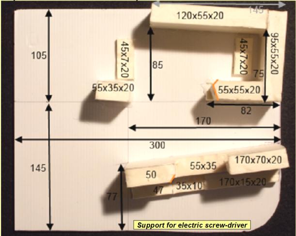
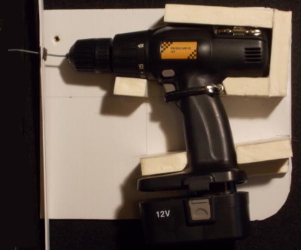
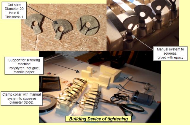
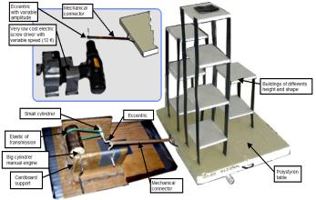
Using electric screw driver
|
|
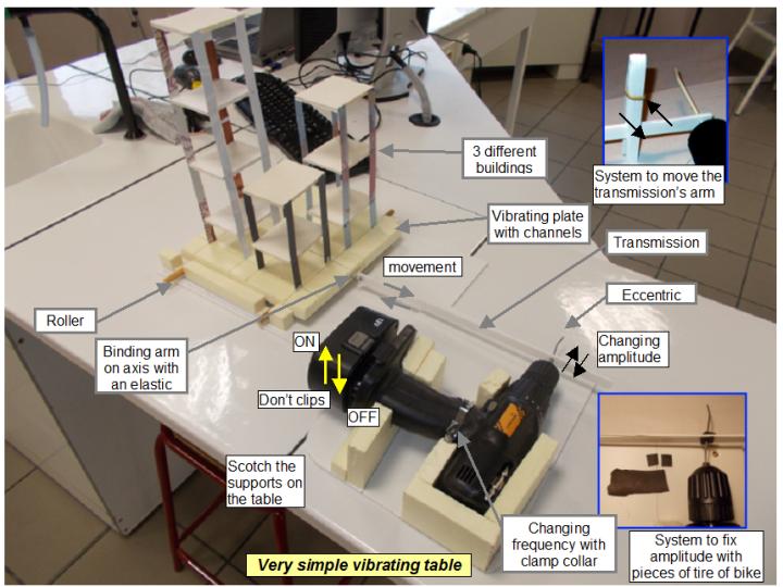
Experimental system:
The electric screw-driver is set on a
support wich is fixed on the table with scotch.
The fréquency is variable by rotating the
screw on the clamp collar.
Using excentric
|
|
|
|
The angle of the eccentric can be change
to limit the vibration amplitude wich is obtained by moving closer or by
taking away the arm of the screwing machine.The system of moving the arm
along the eccentric must be fixed to be sure that the amplitude of the
vibration is the same from one experiment to an other one (to invent)
The screwing machine is started by
raising slightly the battery, and stopped by releasing it.
The vibrating plate must be in the best
position before fixing it.
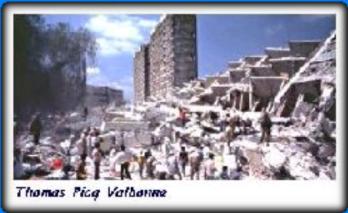
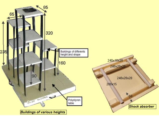
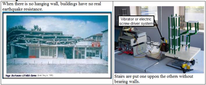
Resonance and building’s size, site
effect.
|
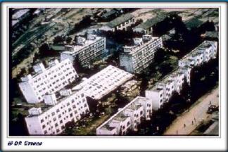
(Mexico earthquake: same dammage in
Mexico than at the epicenter: site effect)
http://www.palais-decouverte.fr/expos/vst_2k7/vs_2k7/pages/page_s6_seisme.html
|
To understand picture as this, where
the small buildings (5 stairs)
collapsed and not the big (15 stairs), it is necessary to study the
resonance.
|
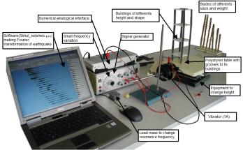
What frequencies present in a
earthquake?
The sofware Simul_seismes©FT
freeware makes the Fourier transforma of an earthquake traces:
You can acceed to this sofware from ![]() .
.
Open the file 95090804.ASC (08 september 95 near
Grenoble) right click /Fourier Total
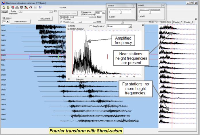
On the right Fourier transform of all
stations (abscissa: amplitude, ordina: fréquencies). On the center the
selected station.
This Fourier transformation shows that
more far from the epicenter we are, more the hight frequency desappears and
the low frequencies are present (as the trumpeting of the elephant wich can
be eared very far away because of it’s very low frequencies)
We can see also that for certains stations,
certains frequencies are amplified.
The conclusion is that for certain
earthquakes, it is possible to see an amplification of certain frequencies
(site effect or other phenomenons ?)
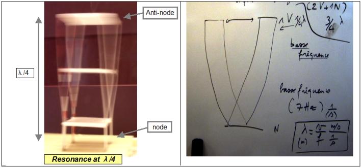
Testing resonance on shaking table:
Higth frequencies make resonate small
buildings and low frequencies make resonate hight buildings.
This phenomenon is not proportional. It
depends of the wave speed in the building.
With the screwing machine, change the
fréquency and obsere the amplitude of each building. The amplitde of the
stimulation must not be to big (buildings collapse when fundations are not
resistant enough).
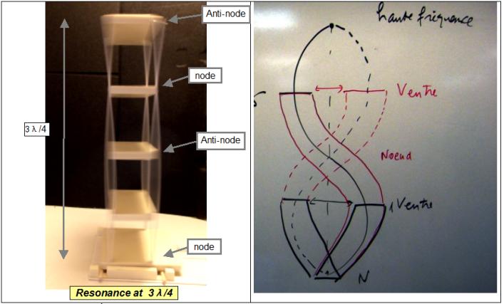
2 vibrating modes are seen:
|
|
 (Photos were made in low light without
flash with a tripod)
(Photos were made in low light without
flash with a tripod)
The second mode is observed on the big
building and the height frequency
The foresters say that in
case of storm, trees break in 1/3 of their height. (in the position of the
antinode)
A little of theory
à For the vibrating blades of length L with a
free extremity, the blade being fixed at the other end, the modes of
vibrations of the blade in the resonance ( maximal amplitude) are such as:
-
There
is a body of vibration at the end of the blade
-
L =
( 2 k + 1) l/4
in using the relation l
= V T = V / N we
deduct that:
first mode : k = 0 , L = l / 4 , N = V / 4 L,
We observe a node and a body on the length
L
second mode : k = 1 , L = 3 l / 4 , N = 3 V / 4,
we
observe : a node, a body, a node, a body on the length L.
V=speed; N number of nodes; l is the wave length; k=is an
integer which is the range of the vibration.
à If the extremity is fixed (rope) then L = k l / 2 then N = k V / 2 L
We will
reuse it for the site effect.
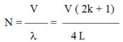
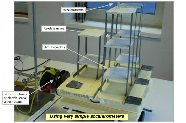
Evaluate the acceleration of buildings
at differents stairs: with a small amplitude.
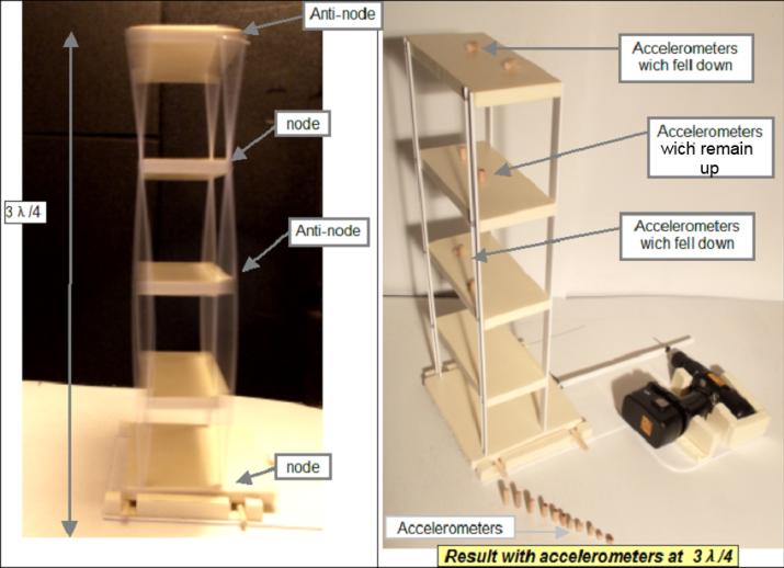
|
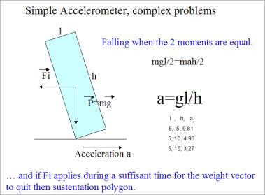
The simple accelerometers: They are constituted by parallelepipeds in Plexiglas of the same
section but of different height which we put at different heights on
buildings and which allow to estimate the acceleration according to the
height of the building and its possible echo. The more the height of the
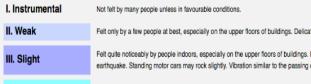
accelerometer is big, the more a low acceleration brings down it. The scale of Mercalli indicates the
awakening of certain persons in the superior floors.
|
l length
of the basis ; h=height ; a=acceleration |
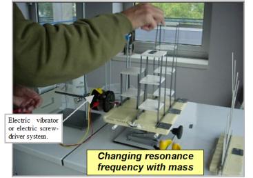
If you put a mass upon a resonating
building, vibration is amorted, and changes for low frequency. You can
retrieve the new resonating frequence by decreasing the frequency.
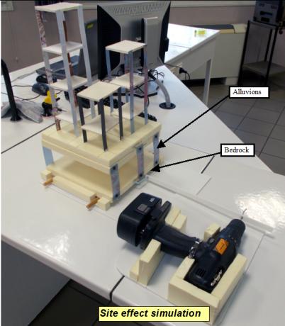
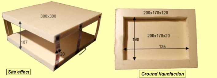
Ground resonance with shaking table (site effect)
|
|
|
We place buildings on a flexible support medium feigning alluvions
and having it’s own resonating frequency; then by changing frequency of
vibration, we succeed in making resound the ground and to amplify very
strongly the amplitude of the initial movement. We apply an horizontal vibration, and we can consider each column of
alluvion as a blade. By reducing the height of the alluvions, we increase resonance
frequency. |
|
Example of site effect (alluvion
Grenoble basin)
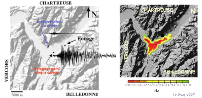
The reality (Pierre-Yves Bard ingenior and researcher Grenoble) shows
that amplitude of the movement is multiplied by 10-20 if we compare with the
amplitude on the rock. If the thickness is important, frequency is low. The
right picture had been done from the noise seismic bottom. Low frequency are
amplified when the thickness of alluvions is important. (red color)
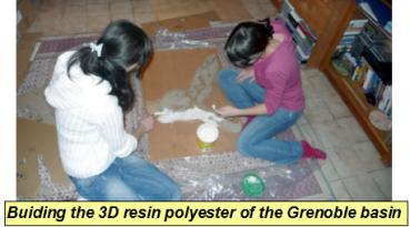
The site effect had been studied thanks to an analogic maquette in resin polyester filled with agar gely. Little pieces of fish food are put into gelly to see the movement. Films are done with 2 differents frequencies, and the pictures of extreme movements are extract from the video and colored in green and red. (DEWEZ Ambre DUMONT Isabelle SERRES Olivia (2010) students in Lycée Marie Reynoard near Grenoble)
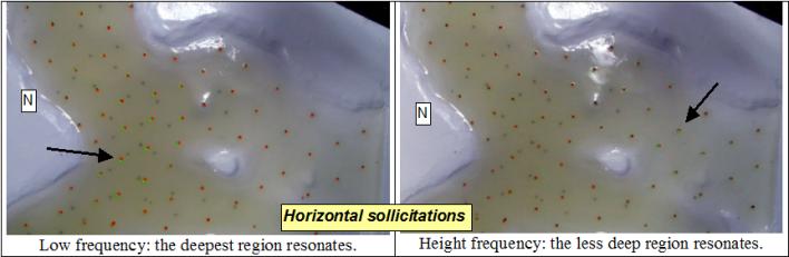
|
|
|
|
Edge of valley resonates with hight
frequencies vibrations.
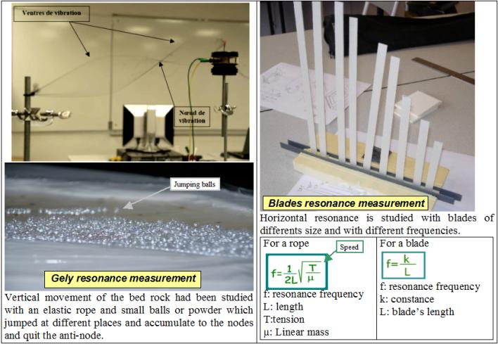
Resonance
of vibrating blades:
Fourier
transform of the sound produced by a rule and recorded with a microphone, or
a piezometer.
The
software Audacity can draw the spectrum of the signal. We have to get the
fundamental frequence (frequence for maximum amplitude). The rule must be
very well fixed on the table.
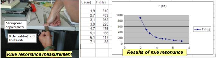
The law
is not proportional, but it is difficult to have the real law, because of the
incertitude on the ruler length. However it is simple to show that the
frequency of the resonance is not proportional with the length of blade.
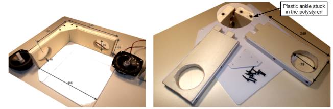
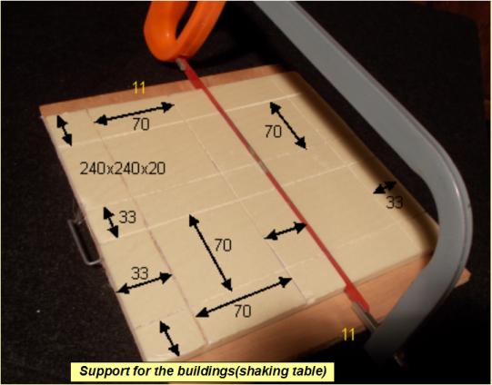
How to build shake table, buildings and supports
for them by yourself?
Reference of this electric screw-driver at
the end of this document.
2 pieces of wood allow to sink not too much
into the polystyren
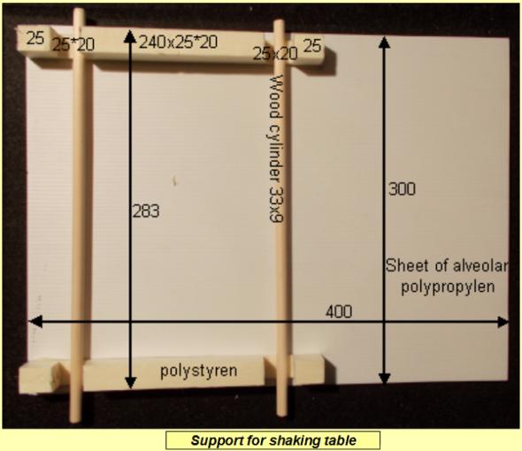
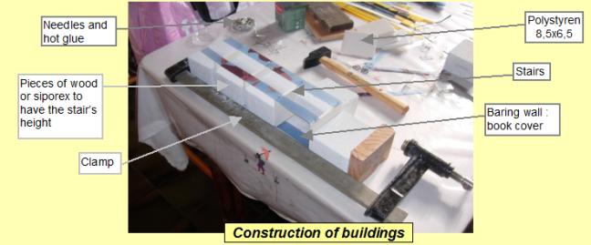
How to build shake table,
buildings and supports for them by yourself?
Buildings
are done with the cover of exercice book, thin polystyren, a guillotine,
needles and hot glue.
How to build an electronic
1D-2D shaking table?
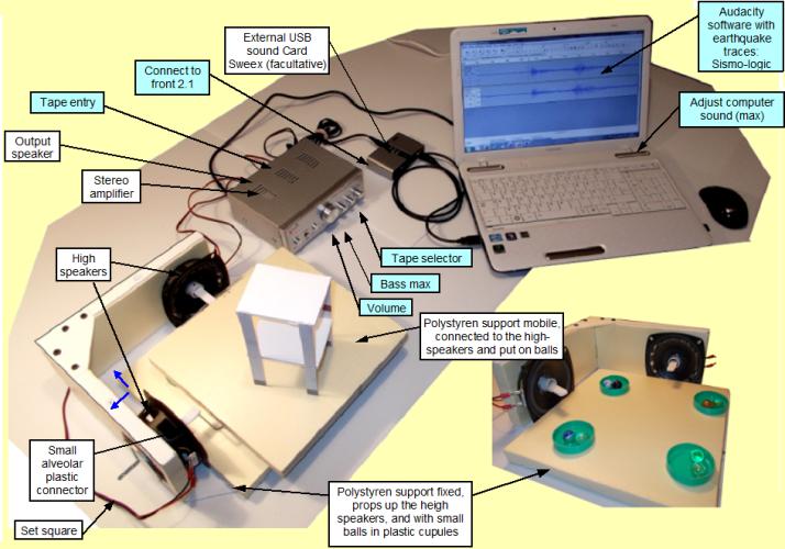
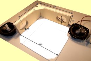
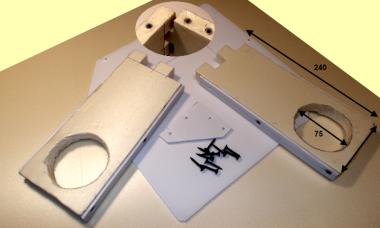
|
|
Necessary equipment to make this experiment:
(Conrad) Dynavox mini-ampli Hi-Fi CSPA1 silver ref :76001
1 F7 39,90 € 2*High
speakers SPEAKA HP 75-9 ref: 300237 1 F7 2*12,95 € USB
external sound card 7.1 USB2.0 ref: 87176 1 F7 39,95 € The high speaker can be perforated to
increase the movement amplitude, but the external sound-card is very efficient,
particulary with laptop computers. The main interest using a
electronic shaking table, is to send to the table a real earthquake trace,
and to approach the reality. In a real trace, all frequencies as present
and the building resonance shows that phenomenon. This system allows also to send relative high frequencies usefull to study building resonance in 3λ/4 mode. |
Using the electronic shaking table with audacity:
- You
need a real earthquake traces (3D eventually) to use this system, with a near
earthquake.
- After
you have to convert this trace in .wav file to use Audacity.
Getting
a 3D .wav trace of an earthquake:
With
sismo-logic run the item “Audacity for shake table 1D-2D” and good files will
be loaded in Audacity.
Making
a 3D .wav trace of an earthquake
- Connect
to http://www.edusismo.org then flag
English, Seismic data, Seismogramms selected, Choose fom the list, 2010,
Confirm, 08/07/2010 SSE MANOSQUE (04), click on the eye.
![]()
- Then
choose NICF station, and downlad the 3 components Z.SAC, N.SAC, E.SAC
(vertical, north, east)
![]()
- You
have now to convert .SAC file in .WAV file for audacity with Seisgram2K
software.
Download
Seisgram2K on http://www.edusismo.org
, “Educational Resources”, “Acess to media ressource”.
In
seisgram2K menu Fichier, Selectionner Fichier…, multiselect your 3 files with
Shift-click ,Button Ouvrir.
|
|
The 3 traces appear in Seisgram. Then take menu « Fichier », « Enregistrer actif
sous », Wave file in « Fichier du type », and choose a
directory and a name. Seisgram add “Composante0, composante1, composante2,
format Wav and PC_INTEL button « Enregistrer ». Seisgram ask for the
multiplicator frequency: choose 1 for the initial frequency or 2, 3, 4 to
increase the speed. It is sometimes necessary to increase frequency because
certain sound cards do not know how to sort infra- sound waves. (<20 Hz)
You have now 3 Wav files wich can be run with Audacity. |
Using
WAV file with audacity,
|
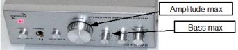
External sound card Sweex
wich must be connected to the computer, before running Audacity and
connected to the amplifier in front 2.1 (facultative using), |
Amplifier dynavox with amplifier button max, bass button max, and
heigh-speakers connected back. |
In
Audacity, menu “Fichier”, “Importer” and multiselect with shift click,
manosque_composante1 and 2:
|
|
Click on the left arrow of each trace and put the first trace in
“Canal gauche” (left channel) and the second trace in “Canal droit” (right
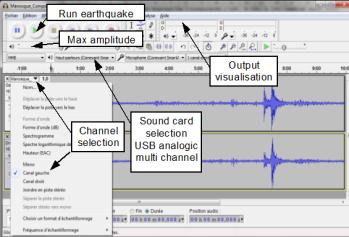
one) If you have the external sound card, select it. Select the maximum amplitude for Audacity output, and verify that
the computer sound is on et is maximum. Put the cursor just before earthquake, and read the sound with the
classical green button. You can simulate differents magnitude, in changing the amplification
with Windows, Audacity, or the Dynavox amplifier button. |
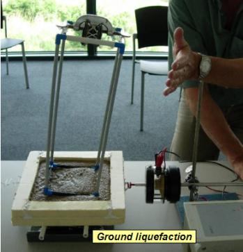
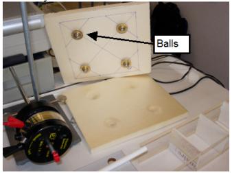
Ground liquefaction and fundations.
|
|
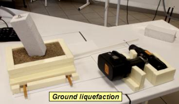
Buildings are built well, but the
heterogeneousness of the foundations causes their collapsing.
|
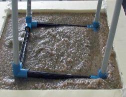
The results are better when the
foundations are reduced to segments as it is often the case in reality. It is necessary to put some sand and
to moisten it. We observe that the water rises and that the building
collapses if the basement is heterogeneous. The objective of the engineers will be
to verify the homogeneity of the basement.
|
|
XI) TESTING EATHQUAKE RESISTANCE SYSTEMS
![]()
When the hazard is known the risk
depends on the building fragility. The earthquake-resistance of the buildings
decreases the risk.
|
|
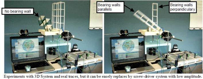
Bearing
walls must fom top to botom of the building and be perpandiculary.
|
|
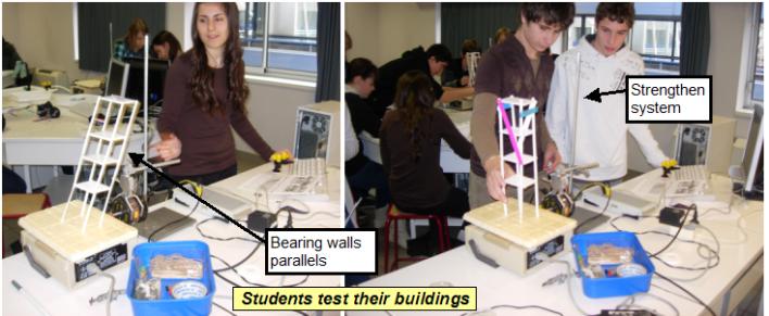
The goal for these students is to make
buildings with wall and staires and with only 4 pins by stair. If bearing
walls are parallel the building does not stand, and after several tries it is
necessary to strengthen it.
They can test their buildings on shaking
tables.
Rolling fundations:
|
|
The principle is
to isolate the building from the ground.
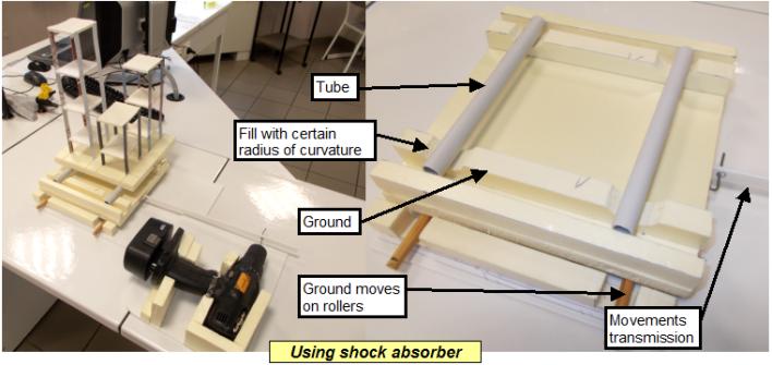
The movements of the ground are
weakened, and it is particulary visible on height frequencies, but we can see
an amplification on low frequencies (resonating of the weakened system), wich
is not the searched effect.
|
Denis DAVI CETE
Méditerranée (p75) |
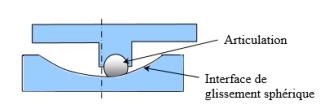
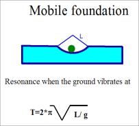
It is
easily demonstrable (by the experiment), that this system can be likened to
an inverted heavy pendulum and that the frequency of resonance can find
itself by the classic formula.
The
main difficulty is to make the lower half-sphere |
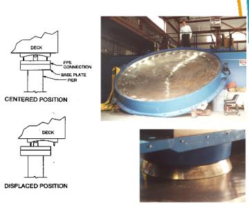
Source:
http://www.cotita.fr/IMG/pdf/JT_seisme_2012_J2_2_Conception_parasismique_ponts_1_Analyses_V3.pdf
Triangulated contreventement
|
|
The construction
is not good and has to be reinforces with triangulated system.
|
|
Triangle is not
deformable
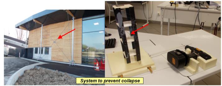
The model of building must be built with
a single pin by floor and the parallel bearing walls. We can add a lead small
piece above to favor the instability. Without contreventement, the building
collapses when it is submitted to an earthquake. After strengthening, the
building remains standing.
|
|
|
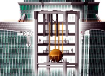
87th Floor Taipei tower From
Wikipedia, the free encyclopedia |
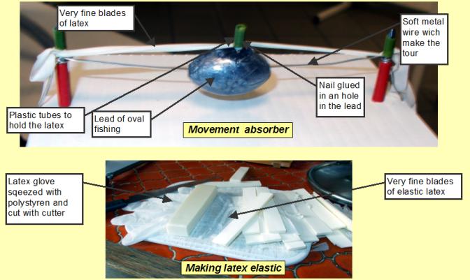
Movement absorber Leaky plate of Manilla paper is
pearced with two nails. A wire, in which a lead of 75 g passes, is
tightened between the two nails. An elastic returns the lead in its equilibrium
position. The set is fixed at the top of the
building. When the building moves, the lead
tends to remain immovable. The elastic stretches and returns the building
in its initial position, what limits its movement. |
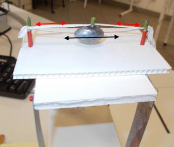
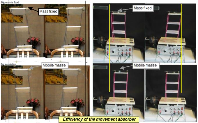
We search the resonance frequency when
the mass is fixed, then we release the mass and we see the amplitude of the
movement which decreases.
The mass size has probably an influence,
and the steepness of the elastic too. Results seems to be better with a small
mass and a very lung elastic. Those parameters can be tested.
How to build movement absorber by yourself?
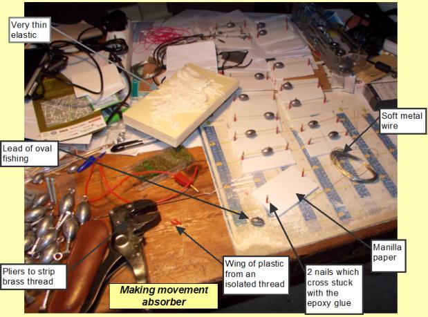
The
resonance frequence of the building must be probably very different than the
frequnce of the movement absorber. We have not tested enough this movement
absorber to be able to define it’s best characteristics.
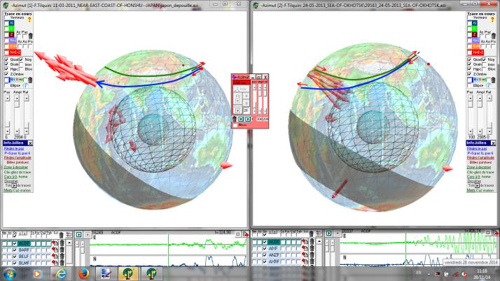
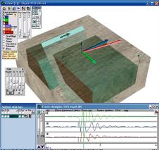
XII) MOVEMENTS OF THE 2 SIDES OF
A FAULT with
Azimut software: ![]()
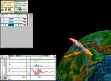
Example
of Japan: read all earthquakes of japan, and click on the first check general
Gn to have the main arrow. What king of movement in Europe? Japan goes on the
pacific, an we have gone at the opposite direction why ? Fault in japan and
opposite movements in France.
Earth
rotondity and slope of the fault make that Europa felt first the pacific
movement and not the Japan movement. So we have the proof than the movements
on both sides of the fault are opposite.
|
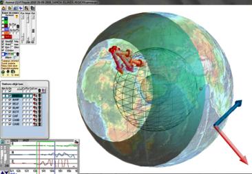
Superficial
Japan earthquake: first movement of France was up. |
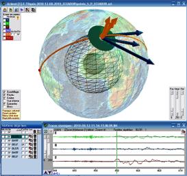
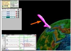
Deep
Earthquake in Okohtsk sea: same fault
movement, but deeper and closer from France. The first movement of
France was down. |
|
|
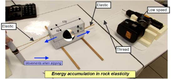
Simulation
of the 2 opposite movements from one side to the other of a fault, with 2
blocks, 2 elastics and the electric screw-driver. The movement is regular,
and forces accumulate, until the slipping.
|
|
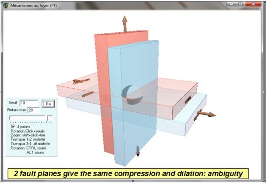
Sofware
“Mecanismes au foyer” modelizes this phenomenon and explains the ambiguity of
the representation mode of faults mechanism.
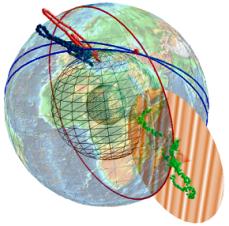
XIII) AZIMUT© FT
12/2011 FREE SOFTWARE
![]()
Goals: The
software shows the 3D ground movments from the 3 components earthquake
stations. The software shows ground speed vector, P, S and L waves, and the
vector extremity with small balls. Epicenter can be found also with tools
wich uses the vector extremity and the user decides the best direction.
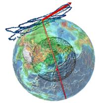
Why do japan earthquake pushed us, althow japan went on the
pacific ocean for few meters?
Samoa eathquake pull us: why?
This software is also able to
record movements of USB accelerometer and is able to drive 1-3 Cassy
interface(s) for a shake table.
|
|
|
|
First
ground movement:
temporary depression (Samoa) |
Perpendicularity
of P-wave and S-wave. 1st
arc pointed. |
|
|
|
|
|
Azimut and
ground compression movement : Japon (1st arc) |
Perpendicularity
of P-S waves (Vector
extremity during few sec) |
Love
wave :S-wave horizontal and perpendiculary to azimut. |


|
|
|
|
|
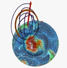
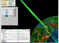
Epicenter
determination with 3 azimuts of P-wave during
10 s. |
Ellipticity
of Rayleigh wave (P-wave perpendic with surface and
azimutal) |
Acquisition of trace from a USB accelerometer. |
|
|
Using Azimut software and “Sismos à l’Ecole” sensor with a small jump
in the school.
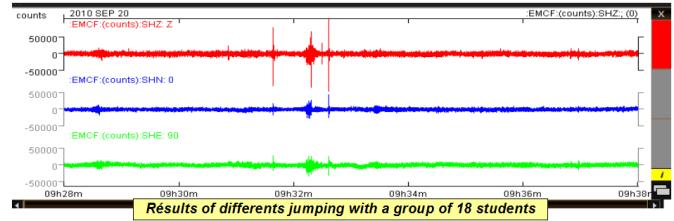
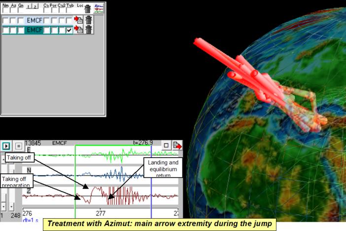
During this last essay, we
find well 3 phases of the jump: the takie-off preparation which is translated
by a movement downward, then the take-off which is translated by a movement
upward and the more or less synchronous exaggerated landing with a sort of
kick-ground which is well translated by a movement downward, with return in
the oscillating balance.
|
“Taking
off” preparation (downward ground movement) |
“Taking off” (upward ground movement) |
“Landing” (downward ground movement) |
Decomposition
of three phases of the jump of the students
Download software Azimut (512 Mo)
XIV) DIFFERENT PEDAGOGICAL SHAKING TABLES
:
![]()
Simple study of BUILDING’S resonance and earthquake
resistance in the classroom.
|
|
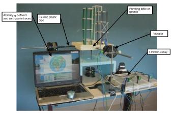
The first
one D pedagogical shake table (nov 2005 CERN Geneva). Real earthquake is send
to Leybold interface by a dedicate software (simul_seismes FT). The a
controlled sinusoïd is sent to the vibrator. Resonance, Amortissor, ground
liquefaction can be shown with this experimental devices.
|
|
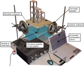
The 3D
shake table consist in 3 loud speakers connected with 3 numerical- analogical
Leybold interfaces, connected to the computer. The signal is a real 3D
earthquake vibrations sent to the interface by the Azimut free-software.
|
|
The building is a spring and we can see the lateral
scissoring and the waves climbing in it from the ground.
|
|
Very basic shaking table with an electric screw-driver, an excentric,
and a clamp collar to hing the speed button.
These experiments simulate seismic vibrations
on very simple plastic buildings, more or less good built, with or without
bearing walls or fundations, chaining or not, put on rolling fundations.
It is possible to study resonance of
differents various height buildings, resonance of the ground as alluvions
valley, in using differents vibrations systems and a lot of other problems.
|
The lower
cost shake table (from
0 € to 12 €): only
sinusoïdes vibrations |
The shake
table built with an old stereo equipment (sinusoïdes and earthquakes vibrations). |
|
The first
peagogical shake table
presented at Science on stage nov. 2005 (sinusoïdes and earthquakes) |
The 3D pedagogical shake table
(sinusoïdes and earthquakes)
|
|
Shake table
built with simple electronic equipement (sinusoïdes
and earthquakes) (110
€) |
|
Download softwares and
applications :http://www.ac-grenoble.fr/webcurie/sismo/web_patin
Scientists: Pierre-Yves
BARD (Searcher
IFSTTAR), Michel CARA (CNRS BCSF Strasbourg),
Françoise COURBOULEX (CNRS UMR Geoazur, Valbonne), Francesca CIFELLI (Dipartimento
di Scienze Geologiche, Roma Tre), Filippo CAMERLENGHI & Lucas MARIANI (Video), Fabrice
FINOTTI (Les Films Associés), François THOUVENOT
(CNRS LGIT Grenoble).
Important
remarks:
If some
people see errors or critics, send them to me: francois.tilquin.38@gmail.com
Say too
if you have difficulty to use the Sismo-box “do it yourself”. Thanks.
XV) COST TO BUILD THE SISMO BOX “DO IT YOURSELF” IN
€ ![]()
|
Réf :
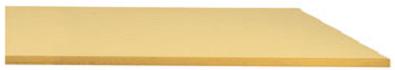
952463 Castorama; 2*(
Polystyrènes extrudé BD 1,25m x 0,60 m ép.20mm ; Unit 1,88 €) |
(for all supports: shake table,
liquefaction, seismometer…) |
3,76 |
|
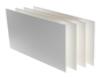
Réf. : VMP0111 VPC display Plaque
Polypro blanc ¼ *( Alvéolé 80 cm*120 cm ep :3mm Unit 2.03€) |
|
0,5 |
|
Réf: 456988 http://www.rougier-ple.fr 1/12*( Carton mousse-plumes 50x65cm ep :5mm Lot de 4 :17,5€) |
|
1,5 |
|
1*( Cahier classeur
Casino 2 .95 €) |
|
2,95 |
|
1/19 *(Epingles patafix
élastique 1 € Buro+ 28,5 € 20,85 €) |
(to build buildings and fix stairs at
walls) |
2 |
|
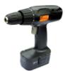
Réf : 488105 Castorama 1*
(Perceuse sans fil 12 V HP12CD. 12,9 €) |
|
12,9 |
|
Réf : 592896 Castorama 0,5*( 2 colliers de serrage inox L8 x ø 32 – 52 Unit :3,69
€) |
|
1,84 |
|
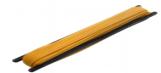
Réf
: 811345 ; Castorama ¼ (Tube IRL tulipé gris. Ø : 16 mm. Long:
2 m. Unit 0,9 €) |
|
0,2 |
|
Réf : 811347 ; Castorama ½ (Tube IRL tulipé gris. Ø : 20 mm. Longueur : 2 m Unit 1,1 €) |
|
0,6 |
|
1/19 *(Tourillon Hêtre 1.5 €, 0,8 cm et 0,9 cm Tourillon sapin 10.5 €) |
|
1,5 |
|
Réf : 123401 Castorama
22/20 * (Vis plaque de plâtre 3,5*25 1,5€ les 20) |
|
1,5 |
|
Réf : 123509 Castorama 2 /20 * (3,5x55 2,7€ les 20) |
|
0,27 |
|
Réf : 634175 Castorama 1/10
*(Tire-fond acier zingué 2,45€) |
|
0,24 |
|
Réf : 110562 Castorama 1/10*(10
Boulons tête fraisée acier zingué 4 x 50 mm 2,45€) |
|
0,24 |
|
Réf : 110442
Castorama 1/10*(10 Écrou hexagonal acier zingué Ø 4
mm 1,5€)
|
|
0,15 |


|
Réf :
634310 Castorama 1/100 (100 Pointes tête plate 3.4
x 80 mm unit 2,6 €) |
|
0,03 |
|
Réf : 634277
Castorama 1/100*(100 Pointes tête plate 2.2 x 40 mm
unit :2,6€) |
|
0,026 |
|
Réf : 634271 Castorama 2/100
Pointes
tête plate 1.4 x 25 mm unit : 2,6 €) |
|
0,052 |
|
Réf :4595
16/50*( Cheville - lot de 50 - vert - 7x35 mm Unit. 3,75 €) |
|
1,2 |
|
Réf : 579076 Castorama 0,5* (Lot de 2 bandes 100 x 610 mm – assortim. MAC ALLISTER. Unit 9,9
€) |
|
4,45 |
|
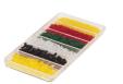
Réf : 552384 Castorama 1*(
Boîte de rangement Kliker violet 35L. L:57
x l:39 x h:20,5 cm. Capacité
: 35L.unit 10,9€) |
|
10,9 |
|
Réf : 224450 ; Décathlon 2/3*( Plomb olive bombée percée 75g CAPERLAN Unit 2,29 €)
|
|
1,52 |
|
Réf: 618068; Décathlon 1/8 *(Zim fluo elastic
Unit 2,75 €) |
|
0,35 |
|
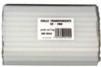
Réf : 264156 Castorama 1/19 *(2 *Colle transparente sachet 1kg Bâtons de colle à chaud. Unit 12,8 €) |
|
1,34 |
|
Réf:
1605262 ; Décathlon 1/10* (Boite assortie gaine Unit 4,95€) |
|
0,5 |
|
Elastiq, règle,
scotch Casino 1,5 € |
|
1,5 |
|
Réf :543470 : Casto L.62,5 h.25 Ep 5cm. Siporex
Concrete (2/16)*1,25€
|
|
0,15 |
|
Ref : 150401 ¼* (Sandow 10m 6 mm Castorama 8,35 €) |
|
2,08 |
|
Réf : 588263 Conrad 1/19*( FER A SOUDER 20 / 120W 2 10,95) |
|
0,52 |
|
Réf : 120369 Castorama Crochet à vis laiton Ø
2,5 x 10 mm. Lot de 10 1/10 *(2,4) Réf 560236 2*(Equerre acier 80 mm 0,85€) |
|
2 |
|
Ref : 710318
Conrad 2 *(
Cordons Jack 3.5 Mm Stereo Droit K3,5S/1,20 Unit 1,6 €) |
|
3,2 |
|
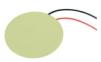
Réf
710397 Conrad 2 *(Transducteurs Céramique Piézo
Epz-27Ms44W 190051 unit 0,63 €)
|
|
1,24 |
|
Réf : 154296 Castorama 1/19 *( Rondelle plate large inox A4. Dimensions : Ø 6 mm. En sécurisac
de 28 pièces. 5,62 €) |
|
0,3 |
|
Réf : 155929 Castorama ¾ (Sangle d'arrimage
polypropylène avec came à griffes 5 m unit 3,26€) |
|
3 |
|
Réf : 609755 Castorama 1/10*( Colle époxy rapide SADER. Unit
8€) |
|
0,8 |
|
Réf :
185106
Conrad 2*
Petit aimant-puissant-permanent-PIC-M0805 unité :1,35 € |
|
2,7 |
|
Réf :
242536
Conrad 1*(Fil de cuivre peint 0,15 mm incolore Mayerhofer
Modellbau) |
|
4,8 |
|
(Earthquake’s location in classroom Réf: 731471
Conrad :10* (Jack
3,5 mm 2 p. unit:0,45€) Réf: 731498 Conrad :10*
(Jack 3,5 mm 2 p. unit: 0,45€) Réf:
604934 Conrad: 17/50 *(wire 50m 0.75mm unit 18,95€) |
(to simulate an earthquake in the classroom
and locate it with 5 stations) |
(15,5) |
|
|
Sum |
70 € |


 (to
close and carry the sismo-box)
(to
close and carry the sismo-box) 
Additional equipement
for the electronic shaking table and experiments with laptop computer
|
Réf: 87176; 1*(Conrad
USB 2.0 external sound card Sweex. Stereo acquisition for wave speed
and good amplification of low frequencies etc…) |
|
39,95 |
|
Réf : 062563-62 ou 76001 ; 1*(Conrad Dynavox mini-amplifier Hi-Fi CSPA1 silver ) |
|
39,90 ou 49,95 |
|
Réf: 300237; Conrad 2*(High speakers SPEAKA HP 75/90 à unit:12,95 €) |
e-shake table) |
25,9 |
|
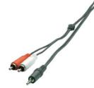
Réf :
325090 ; Conrad 1*(Connexion RCA / jack, 2 m 4,7 € to
connect sound-card to the amplifier) |
|
4,7 |
|
|
Sum |
110,60 € or 120 € |
 (to
amplify output signal of the sound card to the high-speakers of the e-
shake table)
(to
amplify output signal of the sound card to the high-speakers of the e-
shake table)
 (to
connect sound card to the amplifier)
(to
connect sound card to the amplifier)
XVI
DOWNLOAD SOFTWARE
![]()
(automaticly unzipped in \sismobox and run with
\sismobox\sismo-logic.exe )
you can copy the \sismobox folder on a usb-key and run with
\sismobox\sismo-logic.exe
|
1_sismo-logic_ULTRA-LIGHT : basic software with Audacity portable, which set Audacity for parameters for differents experiments, and treats data of stick slip experiment. |
1_sismo-logic_ULTRA-LIGHT.zip (98 Mo) |
|
2-sismo-logic_ULTRA_LIGHT_doc : doc and powerpoints documents wich explains differents functionality and how to build sismobox « do it yourself » |
2-sismo-logic_ULTRA_LIGHT_doc.zip (219 Mo) |
|
3_sismo-logic_software_azimut :AZIMUT software wich treats 3D components. |
3_sismo-logic_software_azimut.zip (512 Mo) |
|
4_sismo-logic_dossiers_films : differents films and software to use with the sismobox |
4_sismo-logic_dossiers_films.zip (408 Mo) |
|
5_sismo-logic_softwares_edusismo : 2 free softwares of Edusismo.org site. |
5_sismo-logic_softwares_edusismo.zip (593 Mo) |